Lightnews — Scholar-powered news

Madison Chapel @chapelmadison.bsky.social · Sep 3

12/ For more results and full details on the simulation framework, take a look at our preprint! www.biorxiv.org/content/10.1...

Evolutionary simulations reveal role for genomic recombination in the evolution of gene regulatory network complexity and robustness

The gene regulatory networks (GRNs) of eukaryotes are dramatically more complex than the GRNs of prokaryotes, but we lack a complete picture of the selective pressures that have shaped this difference...

www.biorxiv.org

Madison Chapel @chapelmadison.bsky.social · Sep 3

11/ Our simulations suggest that, rather than being a direct target of selection, GRN complexity may arise as a byproduct of other evolutionary processes. And to close things out, here’s an animation of a GRN evolving. Watch how fitness and complexity change as the population evolves ! 🎥

1

Madison Chapel @chapelmadison.bsky.social · Sep 3

10/ We saw that complexity emerged more rapidly under changing environmental conditions. For recombining populations, this effect was particularly pronounced.

1

Madison Chapel @chapelmadison.bsky.social · Sep 3

9/ We simulated changing environments by shifting the expression goal for a subset of genes. You can see fitness decrease sharply as the environment changes, followed by recovery as populations adapt.

1

Madison Chapel @chapelmadison.bsky.social · Sep 3

8/ Recombination also modulated the rate at which complexity emerged. In static environments, recombination delayed the emergence of complexity – likely by purging deleterious mutations and slowing drift. But real environments are rarely static !

1

Madison Chapel @chapelmadison.bsky.social · Sep 3

7/ So what did recombination do? First off, recombining populations were consistently more 𝗿𝗼𝗯𝘂𝘀𝘁 than non-recombining ones – they were better at maintaining an expression profile after mutational perturbation. This matches observations from many previous studies!

1

Madison Chapel @chapelmadison.bsky.social · Sep 3

6/ When all other factors are matched, recombining and non-recombining populations converge, rather than diverge, in complexity. This suggests that the complexity 𝘭𝘪𝘮𝘪𝘵 may be defined not by the reproductive strategy but by other features of the GRN system, which we held constant.

1

Madison Chapel @chapelmadison.bsky.social · Sep 3

5/ Surprisingly, recombination didn’t change the final complexity. Neither mutation rate nor initial binding affinity mattered, either. Given enough time, everything converged to ‘random’ GRN complexity; the same level seen in populations evolved 𝘄𝗶𝘁𝗵𝗼𝘂𝘁 𝗮𝗻𝘆 𝘀𝗲𝗹𝗲𝗰𝘁𝗶𝗼𝗻.

1

Madison Chapel @chapelmadison.bsky.social · Sep 3

4/ To investigate this, we built a biochemically-inspired GRN model. TF affinities and concentrations determine gene expression. The closer expression levels are to a specific goal, the more fit a GRN is. Using this model, we simulated 1 million generations of evolution.

1 1

Madison Chapel @chapelmadison.bsky.social · Sep 3

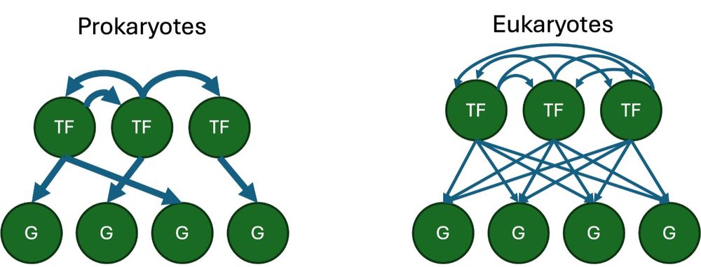
3/ Here’s our idea: complexity in eukaryotic GRNs may have evolved in response to recombination. In simple GRNs, recombination could introduce differently acting transcription factors (TFs) that alter gene expression. In complex GRNs, expression would be buffered by additional TFs

1

Madison Chapel @chapelmadison.bsky.social · Sep 3

2/ Prokaryotic GRNs are relatively simple – there’s specific binding between TFs and their target sites. But in complex eukaryotic GRNs, TFs recognize identical sites throughout the genome, and expression of any one gene depends on multiple TFs binding in combination.

1

Madison Chapel @chapelmadison.bsky.social · Sep 3

1/ Why are eukaryotic gene regulatory networks (GRNs) so much more complex than prokaryotic ones?
In our new preprint, we investigated the role that recombination – a key step in eukaryotic reproductive strategies – plays in this problem! www.biorxiv.org/content/10.1...

Evolutionary simulations reveal role for genomic recombination in the evolution of gene regulatory network complexity and robustness

The gene regulatory networks (GRNs) of eukaryotes are dramatically more complex than the GRNs of prokaryotes, but we lack a complete picture of the selective pressures that have shaped this difference...

www.biorxiv.org

1 1 5

Madison Chapel @chapelmadison.bsky.social · Sep 3

10/ We saw that complexity emerged more rapidly under changing environmental conditions. For recombining populations, this effect was particularly pronounced.

Madison Chapel @chapelmadison.bsky.social · Sep 3

9/ We simulated changing environments by shifting the expression goal for a subset of genes. You can see fitness decrease sharply as the environment changes, followed by recovery as populations adapt.

1

Madison Chapel @chapelmadison.bsky.social · Sep 3

6/ When all other factors are matched, recombining and non-recombining populations converge, rather than diverge, in complexity. This suggests that the complexity 𝘭𝘪𝘮𝘪𝘵 may be defined not by the reproductive strategy but by other features of the GRN system, which we held constant.

Madison Chapel @chapelmadison.bsky.social · Sep 3

4/ To investigate this, we built a biochemically-inspired GRN model. TF affinities and concentrations determine gene expression. The closer expression levels are to a specific goal, the more fit a GRN is. Using this model, we simulated 1 million generations of evolution.

Madison Chapel @chapelmadison.bsky.social · Jan 12

Thank you!!

1

Madison Chapel @chapelmadison.bsky.social · Jan 8

10/ It’s time to shift how we think about variants – instead of associating each variant with a discrete impact on disease risk, they instead have context-dependent distributions of effects. For more details – and more examples! – check out our preprint! www.biorxiv.org/content/10.1...

Variant effects depend on polygenic background: experimental, clinical, and evolutionary implications

Both rare and common genetic variants contribute to human disease, and emerging evidence suggests that they combine additively to influence disease liability. However, due to the non-linear relationsh...

www.biorxiv.org

1 3

Madison Chapel @chapelmadison.bsky.social · Jan 8

9/ Similarly, the dependence on polygenic background means that selection coefficients for the same variant vary across populations, time, individuals, and environments – instead of a single value, they may be better represented as a distribution.

1 2

Madison Chapel @chapelmadison.bsky.social · Jan 8

8/ Because the same variant has different phenotypic consequences in different genetic backgrounds, it could persist in low-risk backgrounds indefinitely, while being strongly selected against in individuals with high polygenic risk!

1 2

Madison Chapel @chapelmadison.bsky.social · Jan 8

7/ Polygenic background also changes how selection acts! More alleles contributing to a trait widens the genetic risk distribution, increasing selective pressure as individuals are pushed to extremes. Highly polygenic traits lead to smaller, more uniform effect sizes.

A two-panel figure. The first panel shows distributions of polygenic scores for a disease with 500 (green lines), 1000 (blue lines), or 2000 (red lines) SNPs involved in the trait phenotype. Each line follows a normal distribution, but variance increases when more SNPs are involved. The red distributions are wider than the blue distributions, which are wider than the green. The second panel plots the number of SNPs involved in the trait against the variance in the PGS for the simulated population, and shows that variance increases with more SNPs.

1 2

Madison Chapel @chapelmadison.bsky.social · Jan 8

6/ What about in the clinic? Genetic testing for rare variants could be complimented by PGS info to better stratify patient risk. This would help prioritize those at highest risk of disease for early intervention while providing peace of mind to those at lower risk.

1 2

Madison Chapel @chapelmadison.bsky.social · Jan 8

5/ For researchers: selecting cell lines with an appropriate genetic background may be as crucial as choosing the right cell type when characterizing disease-associated variants. Low-risk backgrounds could mask variant effects that would be revealed in other genetic contexts!

1 2

Madison Chapel @chapelmadison.bsky.social · Jan 8

4/ Disease prevalence scales non-linearly with disease liability. A 1-unit increase in PGS leads to very different changes in disease prevalence depending on whether it occurs in a low-risk (green) or high-risk (red) genetic background. Same variant, totally different outcomes!

A two-panel figure. The first panel plots PGS against disease prevalence, and shows that for five different background rates (disease prevalence in reference group), disease prevalence increases drastically at the high end of the PGS distribution. The second panel shows a bar chart comparing the increases in disease prevalence for a variant introduced to a low-risk background (green bars) and a high-risk background (red bars). For all five reference groups, the red bars are much larger than the green bars.

1 3

Madison Chapel @chapelmadison.bsky.social · Jan 8

3/ That’s a pretty straightforward observation, but it has widespread consequences for experimental design, clinical genetics, and evolution. The key idea is that you cannot fully understand a variant’s effect without considering the genetic background it occurs in. Here’s why:

1 2