Fabian Schneider
@fabianschneider.bsky.social
95 followers 120 following 18 posts
Doctoral researcher. Interested in memory, audition, semantics, predictive coding, spiking networks.
Posts Media Videos Starter Packs
Pinned
fabianschneider.bsky.social
🚨 Fresh preprint w/ @helenblank.bsky.social!

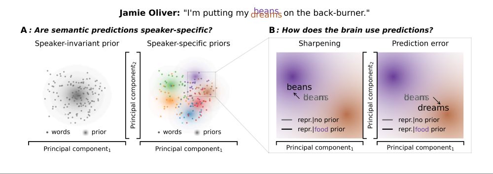
How does the brain acquire expectations about a conversational partner, and how are priors integrated w/ sensory inputs?

Current evidence diverges. Is it prediction error? Sharpening?

Spoiler: It's both.👀

🧵1/16

www.biorxiv.org/content/10.1...
Reposted by Fabian Schneider
lampinen.bsky.social
In neuroscience, we often try to understand systems by analyzing their representations — using tools like regression or RSA. But are these analyses biased towards discovering a subset of what a system represents? If you're interested in this question, check out our new commentary! Thread:
What do representations tell us about a system? Image of a mouse with a scope showing a vector of activity patterns, and a neural network with a vector of unit activity patterns
Common analyses of neural representations: Encoding models (relating activity to task features) drawing of an arrow from a trace saying [on_____on____] to a neuron and spike train. Comparing models via neural predictivity: comparing two neural networks by their R^2 to mouse brain activity. RSA: assessing brain-brain or model-brain correspondence using representational dissimilarity matrices
fabianschneider.bsky.social
Thanks Peter!! :-)

For anyone looking for a brief summary, here's a quick tour of our key findings: bsky.app/profile/fabi...
fabianschneider.bsky.social
🚨 Fresh preprint w/ @helenblank.bsky.social!

How does the brain acquire expectations about a conversational partner, and how are priors integrated w/ sensory inputs?

Current evidence diverges. Is it prediction error? Sharpening?

Spoiler: It's both.👀

🧵1/16

www.biorxiv.org/content/10.1...
fabianschneider.bsky.social
🧵15/16
3. Prediction errors are not computed indiscriminately and appear to be gated by likelihood, potentially underlying robust updates to world models (where extreme prediction errors might otherwise lead to deleterious model updates).
fabianschneider.bsky.social
🧵14/16
2. Priors sharpen representations at the sensory level, and produce high-level prediction errors.

While this contradicts traditional predictive coding, it aligns well with recent views by @clarepress.bsky.social, @peterkok.bsky.social, @danieljamesyon.bsky.social: doi.org/10.1016/j.ti...
Redirecting
doi.org
fabianschneider.bsky.social
🧵13/16
So what are the key takeaways?

1. Listeners apply speaker-specific semantic priors in speech comprehension.

This extends previous findings showing speaker-specific adaptations at the phonetic, phonemic and lexical levels.
fabianschneider.bsky.social
🧵12/16
In fact, neurally we find a double dissociation between type of prior and congruency: Semantic prediction errors are apparent relative to speaker-invariant priors IFF word is highly unlikely given speaker prior, but emerge relative to speaker-specific priors otherwise!
fabianschneider.bsky.social
🧵11/16
Interestingly, participants take longer to respond to words incongruent with the speaker, but response times are a function of word probability given the speaker only for congruent words. This may also suggest some kind of gating, incurring a switch cost!
fabianschneider.bsky.social
🧵10/16
So is there some process gating which semantic prediction errors are computed?

In real time, we sample particularly congruent and incongruent exemplars of a speaker for each subject. We present unmorphed but degraded words and ask for word identification.
fabianschneider.bsky.social
🧵9/16
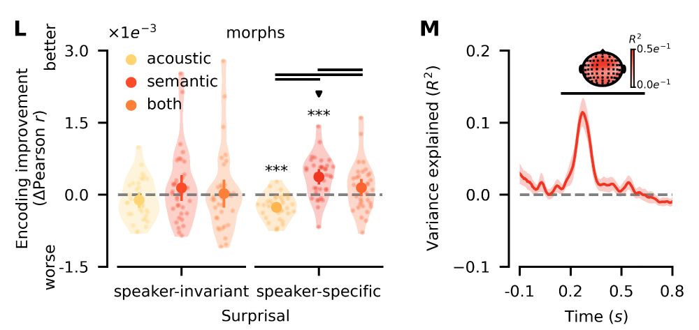
Conversely, here we find that only speaker-specific semantic surprisal improves encoding performance. Explained variance clusters across all sensors between 150-630ms, consistent with prediction errors at higher levels of the processing hierarchy such as semantics!
fabianschneider.bsky.social
🧵8/16
What about high-level representations? Let's zoom out to the broadband EEG response.

To test for information theoretic measures, we encode single-trial responses from acoustic/semantic surprisal, controlling for general linguistic confounds (in part through LLMs).
fabianschneider.bsky.social
🧵7/16
How are they altered? Our RSMs naturally represent expected information. Due to their geometry, a sign flip inverts the pattern to represent unexpected information.

Coefficients show clear evidence of sharpening at the sensory level, pulling reps. towards predictions!
fabianschneider.bsky.social
🧵6/16
We find that similarity structure of sensory representations is best explained by combining speaker-invariant and -specific acoustic predictions. Critically, purely semantic predictions do not help.

Semantic predictions alter sensory representations at the acoustic level!
fabianschneider.bsky.social
🧵5/16
We compute similarity between reconstructions for both speakers and original words from morph creation. We encode observed sensory RSMs from speaker-invariant and -specific acoustic and semantic predictions, controlling for raw acoustics and general linguistic predictions.
fabianschneider.bsky.social
🧵4/16
Let's zoom in on the sensory level: We train stimulus reconstruction models to decode auditory spectrograms from EEG recordings.

If predictions shape neural representations at the sensory level, we should find reconstructed representational content shifted by speakers.
fabianschneider.bsky.social
🧵3/16
Indeed, participants report hearing words as a function of semantic probability given the speaker, scaling with exposure.

But how? Predictive coding invokes prediction errors, but Bayesian inference requires sharpening. Does the brain represent un-/expected information?
fabianschneider.bsky.social
🧵2/16
We played morphed audio files (e.g., sea/tea) and had participants report which of the two words they had heard. Critically, the same morphs were played in different speaker contexts, with speaker-specific feedback reinforcing robust speaker-specific semantic expectations.
fabianschneider.bsky.social
🚨 Fresh preprint w/ @helenblank.bsky.social!

How does the brain acquire expectations about a conversational partner, and how are priors integrated w/ sensory inputs?

Current evidence diverges. Is it prediction error? Sharpening?

Spoiler: It's both.👀

🧵1/16

www.biorxiv.org/content/10.1...
Reposted by Fabian Schneider
danclab.bsky.social
It's been a while since our last laminar MEG paper, but we're back! This time we push beyond deep versus superficial distinctions and go whole hog. Check it out- lots more exciting stuff to come! 🧠📈
maciekszul.bsky.social
🚨🚨🚨PREPRINT ALERT🚨🚨🚨
Neural dynamics across cortical layers are key to brain computations - but non-invasively, we’ve been limited to rough "deep vs. superficial" distinctions. What if we told you that it is possible to achieve full (TRUE!) laminar (I, II, III, IV, V, VI) precision with MEG!
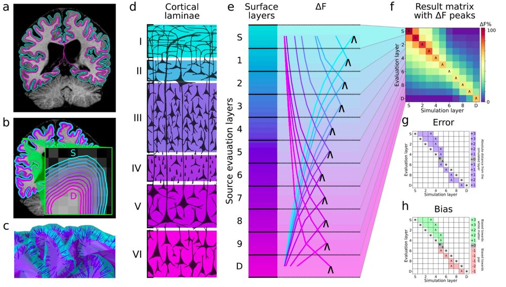
Overview of the simulation strategy and analysis. a) Pial and white matter boundaries
surfaces are extracted from anatomical MRI volumes. b) Intermediate equidistant surfaces are
generated between the pial and white matter surfaces (labeled as superficial (S) and deep (D)
respectively). c) Surfaces are downsampled together, maintaining vertex correspondence across
layers. Dipole orientations are constrained using vectors linking corresponding vertices (link vectors).
d) The thickness of cortical laminae varies across the cortical depth (70–72), which is evenly sampled
by the equidistant source surface layers. e) Each colored line represents the model evidence (relative
to the worst model, ΔF) over source layer models, for a signal simulated at a particular layer (the
simulated layer is indicated by the line color). The source layer model with the maximal ΔF is
indicated by “˄”. f) Result matrix summarizing ΔF across simulated source locations, with peak
relative model evidence marked with “˄”. g) Error is calculated from the result matrix as the absolute
distance in mm or layers from the simulated source (*) to the peak ΔF (˄). h) Bias is calculated as the
relative position of a peak ΔF(˄) to a simulated source (*) in layers or mm.