Interested in microbial genomics, pangenome graphs & evolution 🧬🦠💻
In binary junctions the vast majority of events are gains, often corresponding to an insertion sequence (IS) or prophage integrating in an otherwise conserved region of the genome. This corresponds to a rough rate of one of these events every 20 mutations on the core-genome.

In binary junctions the vast majority of events are gains, often corresponding to an insertion sequence (IS) or prophage integrating in an otherwise conserved region of the genome. This corresponds to a rough rate of one of these events every 20 mutations on the core-genome.
For binary junctions we can go even further: they can be associated with gain or loss events.
In particular singleton junctions correspond to events on terminal branches of the tree, while non-singleton junctions can in principle be associated also to events on internal branches.

For binary junctions we can go even further: they can be associated with gain or loss events.
In particular singleton junctions correspond to events on terminal branches of the tree, while non-singleton junctions can in principle be associated also to events on internal branches.
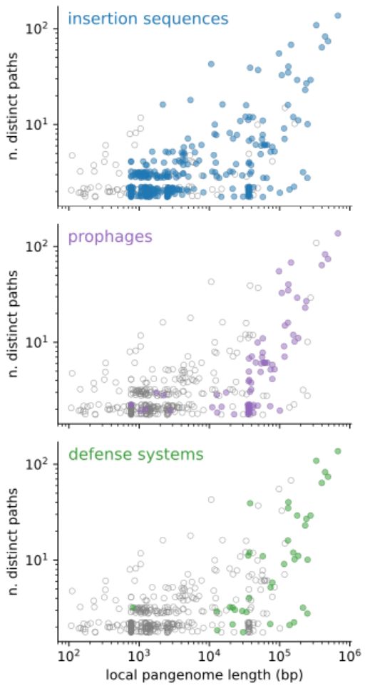
By looking at the content of the junctions, we find that the two peaks in binary junctions are explained by the movement of insertion sequences and prophages respectively, while hotspots are very flexible regions, rich in mobile genetic elements and defense systems.

By looking at the content of the junctions, we find that the two peaks in binary junctions are explained by the movement of insertion sequences and prophages respectively, while hotspots are very flexible regions, rich in mobile genetic elements and defense systems.
If we scatter-plot these two quantities for all of the 519 junctions in the dataset, we find that the majority are binary, i.e. they contain only two possible distinct paths, of which one is often empty. Their length distribution is bimodal, with a peak around 1 kbp and another around 30 kbp.

If we scatter-plot these two quantities for all of the 519 junctions in the dataset, we find that the majority are binary, i.e. they contain only two possible distinct paths, of which one is often empty. Their length distribution is bimodal, with a peak around 1 kbp and another around 30 kbp.
We look at the local graph between two adjacent core blocks, that we call a junction graph. In this graph the diversity can be quantified in terms of number of distinct paths and total accessory sequence content.

We look at the local graph between two adjacent core blocks, that we call a junction graph. In this graph the diversity can be quantified in terms of number of distinct paths and total accessory sequence content.
However, the fact that synteny is largely conserved across big evolutionary distances, and the fact that many of these changes happen on terminal branches of the tree, indicate that these changes are likely removed by purifying selection.

However, the fact that synteny is largely conserved across big evolutionary distances, and the fact that many of these changes happen on terminal branches of the tree, indicate that these changes are likely removed by purifying selection.
Using the graph we can survey all possible changes of synteny in the dataset. Out of 222 isolates, we find only 26 with any change in synteny. Most of these changes are inversions, often around the origin or terminus of replication.

Using the graph we can survey all possible changes of synteny in the dataset. Out of 222 isolates, we find only 26 with any change in synteny. Most of these changes are inversions, often around the origin or terminus of replication.
Once selected the dataset we tackle a second challenge: detecting structural changes. For this we encode all genomes in a pangenome graph. The fundamental units of this representation are blocks, encoding alignments of homologous sequences, and paths, encoding genomes as sequences of blocks.

Once selected the dataset we tackle a second challenge: detecting structural changes. For this we encode all genomes in a pangenome graph. The fundamental units of this representation are blocks, encoding alignments of homologous sequences, and paths, encoding genomes as sequences of blocks.
Thanks to its recent evolution, we can filter out the effects of recombination from the core-genome alignment of this dataset, and recover a reliable phylogeny.

Thanks to its recent evolution, we can filter out the effects of recombination from the core-genome alignment of this dataset, and recover a reliable phylogeny.
Horizontal Gene Transfer, i.e. the exchange of genetic material from one individual to the next, is at the origin of many of these changes. This process however also complicates phylogenetic inference, invalidating the hypothesis of exclusively vertical inheritance.

Horizontal Gene Transfer, i.e. the exchange of genetic material from one individual to the next, is at the origin of many of these changes. This process however also complicates phylogenetic inference, invalidating the hypothesis of exclusively vertical inheritance.
We were motivated by this puzzling observation: microbial genomes can be extremely similar in the core genome, while still differing by large portions of accessory genome.
Therefore we ask:
1) how does this diversity accumulate?
2) at what rate do genomes undergo large structural changes?

We were motivated by this puzzling observation: microbial genomes can be extremely similar in the core genome, while still differing by large portions of accessory genome.
Therefore we ask:
1) how does this diversity accumulate?
2) at what rate do genomes undergo large structural changes?

